All distances between two selections

Here we use distances.distance_array to quantify the distances between each atom of a target set to each atom in a reference set, and show how we can extend that to calculating the distances between the centers-of-mass of residues.

Last executed: May 18, 2021 with MDAnalysis 1.1.1

Last updated: January 2020

Minimum version of MDAnalysis: 0.19.0

Packages required:

• MDAnalysis ([MADWB11], [GLB+16])

• MDAnalysisTests

Optional packages for visualisation:

• matplotlib

import MDAnalysis as mda
from MDAnalysis.tests.datafiles import PDB_small
from MDAnalysis.analysis import distances

import numpy as np
import matplotlib.pyplot as plt
%matplotlib inline

Loading files

The test files we will be working with here feature adenylate kinase (AdK), a phosophotransferase enzyme. ([BDPW09]) AdK has three domains:

• CORE

• LID: an ATP-binding domain (residues 122-159)

• NMP: an AMP-binding domain (residues 30-59)

u = mda.Universe(PDB_small)   # open AdK

Calculating atom-to-atom distances between non-matching coordinate arrays

We select the alpha-carbon atoms of each domain.

LID_ca = u.select_atoms('name CA and resid 122-159')
NMP_ca = u.select_atoms('name CA and resid 30-59')

n_LID = len(LID_ca)
n_NMP = len(NMP_ca)
print('LID has {} residues and NMP has {} residues'.format(n_LID, n_NMP))

LID has 38 residues and NMP has 30 residues

distances.distance_array(API docs) will produce an array with shape (n, m) distances if there are n positions in the reference array and m positions in the other configuration. If you want to calculate distances following the minimum image convention, you must pass the universe dimensions into the box keyword.

dist_arr = distances.distance_array(LID_ca.positions, # reference
                                    NMP_ca.positions, # configuration
                                    box=u.dimensions)
dist_arr.shape

(38, 30)

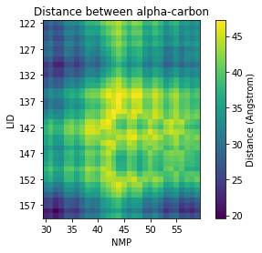
Plotting distance as a heatmap

fig, ax = plt.subplots()
im = ax.imshow(dist_arr, origin='upper')

# add residue ID labels to axes
tick_interval = 5
ax.set_yticks(np.arange(n_LID)[::tick_interval])
ax.set_xticks(np.arange(n_NMP)[::tick_interval])
ax.set_yticklabels(LID_ca.resids[::tick_interval])
ax.set_xticklabels(NMP_ca.resids[::tick_interval])

# add figure labels and titles
plt.ylabel('LID')
plt.xlabel('NMP')
plt.title('Distance between alpha-carbon')

# colorbar
cbar = fig.colorbar(im)
cbar.ax.set_ylabel('Distance (Angstrom)')

Text(0, 0.5, 'Distance (Angstrom)')

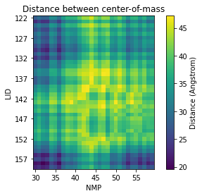
Calculating residue-to-residue distances

As distances.distance_array just takes coordinate arrays as input, it is very flexible in calculating distances between each atom, or centers-of-masses, centers-of-geometries, and so on.

Instead of calculating the distance between the alpha-carbon of each residue, we could look at the distances between the centers-of-mass instead. The process is very similar to the atom-wise distances above, but we give distances.distance_array an array of residue center-of-mass coordinates instead.

LID = u.select_atoms('resid 122-159')
NMP = u.select_atoms('resid 30-59')

LID_com = LID.center_of_mass(compound='residues')
NMP_com = NMP.center_of_mass(compound='residues')

n_LID = len(LID_com)
n_NMP = len(NMP_com)

print('LID has {} residues and NMP has {} residues'.format(n_LID, n_NMP))

LID has 38 residues and NMP has 30 residues

We can pass these center-of-mass arrays directly into distances.distance_array.

res_dist = distances.distance_array(LID_com, NMP_com,
                                    box=u.dimensions)

Plotting

fig2, ax2 = plt.subplots()
im2 = ax2.imshow(res_dist, origin='upper')

# add residue ID labels to axes
tick_interval = 5
ax2.set_yticks(np.arange(n_LID)[::tick_interval])
ax2.set_xticks(np.arange(n_NMP)[::tick_interval])
ax2.set_yticklabels(LID.residues.resids[::tick_interval])
ax2.set_xticklabels(NMP.residues.resids[::tick_interval])

# add figure labels and titles
plt.ylabel('LID')
plt.xlabel('NMP')
plt.title('Distance between center-of-mass')

# colorbar
cbar2 = fig2.colorbar(im)
cbar2.ax.set_ylabel('Distance (Angstrom)')

Text(0, 0.5, 'Distance (Angstrom)')

References

[1] Oliver Beckstein, Elizabeth J. Denning, Juan R. Perilla, and Thomas B. Woolf. Zipping and Unzipping of Adenylate Kinase: Atomistic Insights into the Ensemble of Open↔Closed Transitions. Journal of Molecular Biology, 394(1):160–176, November 2009. 00107. URL: https://linkinghub.elsevier.com/retrieve/pii/S0022283609011164, doi:10.1016/j.jmb.2009.09.009.

[2] Richard J. Gowers, Max Linke, Jonathan Barnoud, Tyler J. E. Reddy, Manuel N. Melo, Sean L. Seyler, Jan Domański, David L. Dotson, Sébastien Buchoux, Ian M. Kenney, and Oliver Beckstein. MDAnalysis: A Python Package for the Rapid Analysis of Molecular Dynamics Simulations. Proceedings of the 15th Python in Science Conference, pages 98–105, 2016. 00152. URL: https://conference.scipy.org/proceedings/scipy2016/oliver_beckstein.html, doi:10.25080/Majora-629e541a-00e.

[3] Naveen Michaud-Agrawal, Elizabeth J. Denning, Thomas B. Woolf, and Oliver Beckstein. MDAnalysis: A toolkit for the analysis of molecular dynamics simulations. Journal of Computational Chemistry, 32(10):2319–2327, July 2011. 00778. URL: http://doi.wiley.com/10.1002/jcc.21787, doi:10.1002/jcc.21787.