Analysing pore dimensions with HOLE2

Here we use HOLE to analyse pore dimensions in a membrane.

Last executed: Feb 20, 2020 with MDAnalysis 1.0.0

Last updated: February 2020

Minimum version of MDAnalysis: 1.0.0

Packages required:

• MDAnalysis ([MADWB11], [GLB+16])

• MDAnalysisTests

• HOLE

• matplotlib

• numpy

Note

The classes in MDAnalysis.analysis.hole2 are wrappers around the HOLE program. Please cite ([SGW93], [SNW+96]) when using this module in published work.

import MDAnalysis as mda
from MDAnalysis.tests.datafiles import PDB_HOLE
from MDAnalysis.analysis import hole2
import matplotlib.pyplot as plt
import numpy as np
%matplotlib inline

Background

The MDAnalysis.analysis.hole2 module (API docs) provides wrapper classes and functions that call the HOLE program. This means you must have installed the program yourself before you can use the class. You then need to pass the path to your hole executable to the class; in this example, hole is installed at ~/hole2/exe/hole.

HOLE defines a series of points throughout the pore from which a sphere can be generated that does not overlap any atom (as defined by its van der Waals radius). (Please see ([SGW93], [SNW+96]) for a complete explanation). By default, it ignores residues with the following names: “SOL”, “WAT”, “TIP”, “HOH”, “K”, “NA”, “CL”. You can change these with the ignore_residues keyword. Note that the residue names must have 3 characters. Wildcards do not work.

This tutorial first demonstrates how to use the MDAnalysis.analysis.hole2.hole function similarly to the HOLE binary on a PDB file. We then demonstrate how to use the MDAnalysis.analysis.hole2.HoleAnalysis class on a trajectory of data. You may prefer to use the more fully-featured HoleAnalysis class for the extra functionality we provide, such as creating an animation in VMD of the pore.

Using HOLE with a PDB file

The hole function allows you to specify points to begin searching at (cpoint) and a search direction (cvect), the sampling resolution (sample), and more. Please see the documentation for full details.

The PDB file here is the experimental structure of the Gramicidin A channel. Note that we pass HOLE a PDB file directly, without creating a MDAnalysis.Universe.

We are setting a random_seed here so that the results in the tutorial can be reproducible. This is normally not advised.

profiles = hole2.hole(PDB_HOLE,
                      executable='~/hole2/exe/hole',
                      outfile='hole1.out',
                      sphpdb_file='hole1.sph',
                      vdwradii_file=None,
                      random_seed=31415)

outfile and sphpdb_file are the names of the files that HOLE will write out. vdwradii_file is a file of necessary van der Waals’ radii in a HOLE-readable format. If set to None, MDAnalysis will create a simple2.rad file with the built-in radii from the HOLE distribution.

This will create several outputs in your directory:

• hole1.out: the log file for HOLE.

• hole1.sph: a PDB-like file containing the coordinates of the pore centers.

• simple2.rad: file of Van der Waals’ radii

• tmp/pdb_name.pdb: the short name of a PDB file with your structure. As hole is a FORTRAN77 program, it is limited in how long of a filename that it can read. Symlinking the file to the current directory can shorten the path.

If you do not want to keep the files, set keep_files=False. Keep in mind that you will not be able to create a VMD surface without the sphpdb file.

The pore profile itself is in the profiles1 dictionary, indexed by frame. There is only one frame in this PDB file, so it is at profiles1[0].

profiles[0].shape

(425,)

Each profile is a numpy.recarray with the fields below as an entry for each rxncoord:

• rxn_coord: the distance along the pore axis in angstrom

• radius: the pore radius in angstrom

• cen_line_D: distance measured along the pore centre line - the first point found is set to zero.

profiles[0].dtype.names

('rxn_coord', 'radius', 'cen_line_D')

You can then proceed with your own analysis of the profiles.

rxn_coords = profiles[0].rxn_coord
pore_length = rxn_coords[-1] - rxn_coords[0]
print('The pore is {} angstroms long'.format(pore_length))

The pore is 42.4 angstroms long

You can create a VMD surface from the hole1.sph output file, using the create_vmd_surface function.

hole2.create_vmd_surface(filename='hole1.vmd',
                         sphpdb='hole1.sph',
                         sph_process='~/hole2/exe/sph_process')

'hole1.vmd'

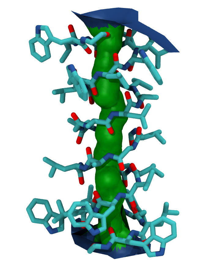
To view this, open your PDB file in VMD.

vmd tmp*/*.pdb

Load the output file in Extensions > Tk Console:

source hole1.vmd

Your pore surface will be drawn as below.

MDAnalysis supports many of the options that can be customised in HOLE. For example, you can specify a starting point for the pore search within the pore with cpoint, and a sample distance (default: 0.2 angstrom) for the distance between the planes used in HOLE. Please see the MDAnalysis.analysis.hole2 for more information.

Using HOLE with a trajectory

One of the limitations of the hole program is that it can only accept PDB files. In order to use other formats with hole, or to run hole on trajectories, we can use the hole2.HoleAnalysis class with an MDAnalysis.Universe. While the example file below is a PDB, you can use any files to create your Universe. You can also specify that the HOLE analysis is only run on a particular group of atoms with the select keyword (default value: ‘protein’).

As with hole(), HoleAnalysis allows you to select a starting point for the search (cpoint). You can pass in a coordinate array; alternatively, you can use the center-of-geometry of your atom selection in each frame as the start.

from MDAnalysis.tests.datafiles import MULTIPDB_HOLE

u = mda.Universe(MULTIPDB_HOLE)

ha = hole2.HoleAnalysis(u, select='protein',
                        cpoint='center_of_geometry',
                        executable='~/hole2/exe/hole')
ha.run(random_seed=31415)

<MDAnalysis.analysis.hole2.hole.HoleAnalysis at 0x10f3f1850>

Working with the data

Again, the data is stored in ha.profiles as a dictionary of numpy.recarrays. The dictionary is indexed by frame; we can see the HOLE profile for the fourth frame below (truncated to the first 10 values).

ha.profiles[3][:10]

rec.array([(-21.01227, 15.3468 , -39.23993),
           (-20.91227, 12.63403, -34.6473 ),
           (-20.81227, 10.63723, -30.05467),
           (-20.71227,  9.58447, -27.7256 ),
           (-20.61227,  8.87309, -25.39653),
           (-20.51227,  8.56876, -23.62047),
           (-20.41227,  8.56275, -21.84441),
           (-20.31227,  8.47622, -21.74275),
           (-20.21227,  8.38983, -21.64108),
           (-20.11227,  8.30039, -21.54024)],
          dtype=[('rxn_coord', '<f8'), ('radius', '<f8'), ('cen_line_D', '<f8')])

If you want to collect each individual property, use gather(). Setting flat=True flattens the lists of rxn_coord, radius, and cen_line_D, in order. You can select which frames you want by passing an iterable of frame indices to frames. frames=None returns all frames.

gathered = ha.gather()
print(gathered.keys())

dict_keys(['rxn_coord', 'radius', 'cen_line_D'])

print(len(gathered['rxn_coord']))

11

flat = ha.gather(flat=True)
print(len(flat['rxn_coord']))

3983

You may also want to collect the radii in bins of rxn_coord for the entire trajectory with the bin_radii() function. range should be a tuple of the lower and upper edges of the first and last bins, respectively. If range=None, the minimum and maximum values of rxn_coord are used.

bins can be either an iterable of (lower, upper) edges (in which case range is ignored), or a number specifying how many bins to create with range.

radii, edges = ha.bin_radii(bins=100, range=None)

The closely related histogram_radii() function takes the same arguments as bin_radii() to group the pore radii, but allows you to specify an aggregating function with aggregator (default: np.mean) that will be applied to each array of radii. The arguments for this function, and returned values, are analogous to those for np.histogram.

means, edges = ha.histogram_radii(bins=100, range=None,
                                  aggregator=np.mean)

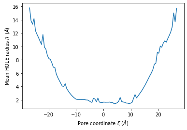
We can use this to plot the mean radii of the pore over the trajectory. (You can also accomplish this with the plot_mean_profile() function shown below, by setting n_std=0.)

midpoints = 0.5*(edges[1:]+edges[:-1])
plt.plot(midpoints, means)
plt.ylabel(r"Mean HOLE radius $R$ ($\AA$)")
plt.xlabel(r"Pore coordinate $\zeta$ ($\AA$)");

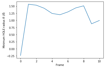
HoleAnalysis also has the min_radius() function, which will return the minimum radius in angstrom for each frame. The resulting array has the shape (#n_frames, 2).

min_radii = ha.min_radius()
min_radii

array([[ 0.     , -0.23655],
       [ 1.     ,  1.56731],
       [ 2.     ,  1.53329],
       [ 3.     ,  1.42503],
       [ 4.     ,  1.2426 ],
       [ 5.     ,  1.19813],
       [ 6.     ,  1.29624],
       [ 7.     ,  1.43776],
       [ 8.     ,  1.51123],
       [ 9.     ,  0.87855],
       [10.     ,  0.99659]])

plt.plot(min_radii[:, 0], min_radii[:, 1])
plt.ylabel('Minimum HOLE radius $R$ ($\AA$)')
plt.xlabel('Frame');

Visualising the VMD surface

The create_vmd_surface() method is built into the HoleAnalysis class. It writes a VMD file that changes the pore surface for each frame in VMD. Again, load your file and source the file in the Tk Console:

source holeanalysis.vmd

ha.create_vmd_surface(filename='holeanalysis.vmd')

'holeanalysis.vmd'

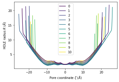
Plotting

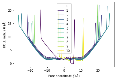
HoleAnalysis has several convenience methods for plotting. plot() plots the HOLE radius over each pore coordinate, differentiating each frame with colour.

ha.plot();

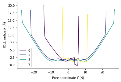
You can choose to plot specific frames, or specify colours or a colour map. Please see the documentation for a full description of arguments.

ha.plot(frames=[0, 2, 5, 9]);

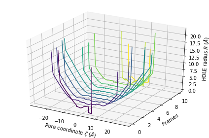
The plot3D() function separates each frame onto its own axis in a 3D plot.

ha.plot3D();

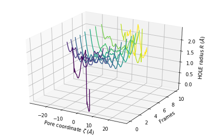
You can choose to plot only the part of each pore lower than a certain radius by setting r_max.

ha.plot3D(r_max=2.5);

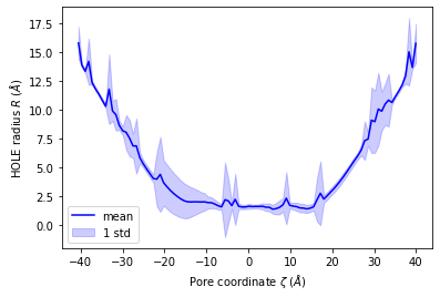
You can also plot the mean and standard deviation of the pore radius over the pore coordinate.

ha.plot_mean_profile(bins=100,  # how much to chunk rxn_coord
                     n_std=1,  # how many standard deviations from mean
                     color='blue',  # color of plot
                     fill_alpha=0.2,  # opacity of standard deviation
                     legend=True);

Ordering HOLE profiles with an order parameter

If you are interested in the HOLE profiles over an order parameter, you can directly pass that into the analysis after it is run. Below, we use an order parameter of RMSD from a reference structure.

Note

Please cite ([SFSB14]) when using the over_order_parameters functionality.

from MDAnalysis.analysis import rms

ref = mda.Universe(PDB_HOLE)
rmsd = rms.RMSD(u, ref, select='protein', weights='mass').run()
rmsd_values = rmsd.rmsd[:, 2]
rmsd_values

array([6.10501252e+00, 4.88398472e+00, 3.66303524e+00, 2.44202454e+00,
       1.22100521e+00, 1.67285541e-07, 1.22100162e+00, 2.44202456e+00,
       3.66303410e+00, 4.88398478e+00, 6.10502262e+00])

You can pass this in as order_parameter. The resulting profiles dictionary will have your order parameters as keys. You should be careful with this if your order parameter has repeated values, as duplicate keys are not possible; each duplicate key just overwrites the previous value.

op_profiles = ha.over_order_parameters(rmsd_values)

You can see here that the dictionary does not order the entries by the order parameter. If you iterate over the dictionary, it will return each (key, value) pair in sorted key order.

for order_parameter, profile in op_profiles.items():
    print(order_parameter, len(profile))

1.6728554140225013e-07 543
1.2210016190719406 389
1.2210052104208637 511
2.4420245432434005 419
2.4420245634673616 399
3.6630340992950225 379
3.663035235691455 443
4.883984723991125 407
4.883984778674993 149
6.105012519709198 205
6.105022620520391 139

You can also select specific frames for the new profiles.

op_profiles = ha.over_order_parameters(rmsd_values, frames=[0, 4, 9])
op_profiles.keys()

dict_keys([1.2210052104208637, 4.883984778674993, 6.105012519709198])

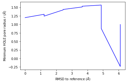
Plotting

HoleAnalysis also provides convenience functions for plotting over order parameters. Unlike plot(), plot_order_parameters() requires an aggregator function that reduces an array of radii to a singular value. The default function is min(). You can also pass in functions such as max() or np.mean(), or define your own function to operate on an array and return a vlue.

ha.plot_order_parameters(rmsd_values,
                         aggregator=min,
                         xlabel='RMSD to reference ($\AA$)',
                         ylabel='Minimum HOLE pore radius $r$ ($\AA$)');

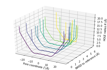
plot3D_order_parameters() functions in a similar way to plot3D(), although you need to pass in the order parameters.

ha.plot3D_order_parameters(rmsd_values,
                           ylabel='RMSD to reference ($\AA$)');

Deleting HOLE files

The HOLE program and related MDAnalysis code write a number of files out. Both the hole() function and HoleAnalysis class contain ways to easily remove these files.

For hole(), pass in keep_files=False to delete HOLE files as soon as the analysis is done. However, this will also remove the sphpdb file required to create a VMD surface from the analysis. If you need to write a VMD surface file, use the HoleAnalysis class instead.

You can track the created files at the tmp_files attribute.

ha.tmp_files

['simple2.rad',
 'hole000.out',
 'hole000.sph',
 'hole001.out',
 'hole001.sph',
 'hole002.out',
 'hole002.sph',
 'hole003.out',
 'hole003.sph',
 'hole004.out',
 'hole004.sph',
 'hole005.out',
 'hole005.sph',
 'hole006.out',
 'hole006.sph',
 'hole007.out',
 'hole007.sph',
 'hole008.out',
 'hole008.sph',
 'hole009.out',
 'hole009.sph',
 'hole010.out',
 'hole010.sph']

The built-in method delete_temporary_files() will remove these.

ha.delete_temporary_files()
ha.tmp_files

[]

Alternatively, you can use HoleAnalysis as a context manager. When you exit the block, the temporary files will be deleted automatically.

with hole2.HoleAnalysis(u, executable='~/hole2/exe/hole') as ha2:
    ha2.run()
    ha2.create_vmd_surface(filename='holeanalysis.vmd')
    ha2.plot()

ha.profiles[0][0].radius

20.0962

References

[1] Richard J. Gowers, Max Linke, Jonathan Barnoud, Tyler J. E. Reddy, Manuel N. Melo, Sean L. Seyler, Jan Domański, David L. Dotson, Sébastien Buchoux, Ian M. Kenney, and Oliver Beckstein. MDAnalysis: A Python Package for the Rapid Analysis of Molecular Dynamics Simulations. Proceedings of the 15th Python in Science Conference, pages 98–105, 2016. 00152. URL: https://conference.scipy.org/proceedings/scipy2016/oliver_beckstein.html, doi:10.25080/Majora-629e541a-00e.

[2] Naveen Michaud-Agrawal, Elizabeth J. Denning, Thomas B. Woolf, and Oliver Beckstein. MDAnalysis: A toolkit for the analysis of molecular dynamics simulations. Journal of Computational Chemistry, 32(10):2319–2327, July 2011. 00778. URL: http://doi.wiley.com/10.1002/jcc.21787, doi:10.1002/jcc.21787.

[3] O S Smart, J M Goodfellow, and B A Wallace. The pore dimensions of gramicidin A. Biophysical Journal, 65(6):2455–2460, December 1993. 00522. URL: https://www.ncbi.nlm.nih.gov/pmc/articles/PMC1225986/, doi:10.1016/S0006-3495(93)81293-1.

[4] O. S. Smart, J. G. Neduvelil, X. Wang, B. A. Wallace, and M. S. Sansom. HOLE: a program for the analysis of the pore dimensions of ion channel structural models. Journal of Molecular Graphics, 14(6):354–360, 376, December 1996. 00935. doi:10.1016/s0263-7855(97)00009-x.

[5] Lukas S. Stelzl, Philip W. Fowler, Mark S. P. Sansom, and Oliver Beckstein. Flexible gates generate occluded intermediates in the transport cycle of LacY. Journal of Molecular Biology, 426(3):735–751, February 2014. 00000. URL: https://asu.pure.elsevier.com/en/publications/flexible-gates-generate-occluded-intermediates-in-the-transport-c, doi:10.1016/j.jmb.2013.10.024.