Average radial distribution functions

Here we calculate the average radial cumulative distribution functions between two groups of atoms.

Last executed: May 18, 2021 with MDAnalysis 1.1.1

Last updated: February 2020

Minimum version of MDAnalysis: 0.17.0

Packages required:

• MDAnalysis ([MADWB11], [GLB+16])

• MDAnalysisTests

Optional packages for visualisation:

• matplotlib

import MDAnalysis as mda
from MDAnalysis.tests.datafiles import TPR, XTC
from MDAnalysis.analysis import rdf
import matplotlib.pyplot as plt
%matplotlib inline

Loading files

The test files we will be working with here feature adenylate kinase (AdK), a phosophotransferase enzyme. [3]

u = mda.Universe(TPR, XTC)

/Users/lily/anaconda3/envs/mda-user-guide/lib/python3.7/site-packages/MDAnalysis/topology/tpr/utils.py:395: DeprecationWarning: TPR files index residues from 0. From MDAnalysis version 2.0, resids will start at 1 instead. If you wish to keep indexing resids from 0, please set `tpr_resid_from_one=False` as a keyword argument when you create a new Topology or Universe.
  category=DeprecationWarning)

Calculating the average radial distribution function for two groups of atoms

A radial distribution function \(g_{ab}(r)\) describes the time-averaged density of particles in \(b\) from the reference group \(a\) at distance \(r\). It is normalised so that it becomes 1 for large separations in a homogenous system.

\[g_{ab}(r) = (N_{a} N_{b})^{-1} \sum_{i=1}^{N_a} \sum_{j=1}^{N_b} \langle \delta(|\mathbf{r}_i - \mathbf{r}_j| - r) \rangle\]

The radial cumulative distribution function is

\[G_{ab}(r) = \int_0^r \!\!dr' 4\pi r'^2 g_{ab}(r')\]

.

The average number of \(b\) particles within radius \(r\) at density \(\rho\) is:

\[N_{ab}(r) = \rho G_{ab}(r)\]

The average number of particles can be used to compute coordination numbers, such as the number of neighbours in the first solvation shell.

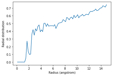
Below, I calculate the average RDF between each atom of residue 60 to each atom of water to look at the distribution of water over the trajectory. The RDF is limited to a spherical shell around each atom in residue 60 by range. Note that the range is defined around each atom, rather than the center-of-mass of the entire group.

If you are after non-averaged radial distribution functions, have a look at the site-specific RDF class. The API docs for the InterRDF class are here.

res60 = u.select_atoms('resid 60')
water = u.select_atoms('resname SOL')

irdf = rdf.InterRDF(res60, water,
                    nbins=75,  # default
                    range=(0.0, 15.0),  # distance in angstroms
                   )
irdf.run()

<MDAnalysis.analysis.rdf.InterRDF at 0x7fee86c56390>

The distance bins are available at irdf.bins and the radial distribution function is at irdf.rdf.

irdf.bins

array([ 0.1,  0.3,  0.5,  0.7,  0.9,  1.1,  1.3,  1.5,  1.7,  1.9,  2.1,
        2.3,  2.5,  2.7,  2.9,  3.1,  3.3,  3.5,  3.7,  3.9,  4.1,  4.3,
        4.5,  4.7,  4.9,  5.1,  5.3,  5.5,  5.7,  5.9,  6.1,  6.3,  6.5,
        6.7,  6.9,  7.1,  7.3,  7.5,  7.7,  7.9,  8.1,  8.3,  8.5,  8.7,
        8.9,  9.1,  9.3,  9.5,  9.7,  9.9, 10.1, 10.3, 10.5, 10.7, 10.9,
       11.1, 11.3, 11.5, 11.7, 11.9, 12.1, 12.3, 12.5, 12.7, 12.9, 13.1,
       13.3, 13.5, 13.7, 13.9, 14.1, 14.3, 14.5, 14.7, 14.9])

plt.plot(irdf.bins, irdf.rdf)
plt.xlabel('Radius (angstrom)')
plt.ylabel('Radial distribution')

Text(0, 0.5, 'Radial distribution')

The total number of atom pairs in each distance bin over the trajectory, before it gets normalised over the density, number of frames, and volume of each radial shell, is at irdf.count.

irdf.count

array([0.000e+00, 0.000e+00, 0.000e+00, 0.000e+00, 0.000e+00, 0.000e+00,
       0.000e+00, 4.000e+00, 2.900e+01, 1.800e+01, 1.600e+01, 2.000e+01,
       8.300e+01, 1.130e+02, 1.080e+02, 1.530e+02, 1.620e+02, 2.090e+02,
       2.430e+02, 2.200e+02, 2.590e+02, 2.690e+02, 3.750e+02, 4.100e+02,
       4.080e+02, 4.760e+02, 4.820e+02, 5.260e+02, 5.630e+02, 6.060e+02,
       6.390e+02, 7.100e+02, 6.780e+02, 7.770e+02, 8.810e+02, 9.440e+02,
       1.003e+03, 1.074e+03, 1.204e+03, 1.237e+03, 1.265e+03, 1.471e+03,
       1.513e+03, 1.526e+03, 1.678e+03, 1.780e+03, 1.782e+03, 2.021e+03,
       1.998e+03, 2.133e+03, 2.309e+03, 2.241e+03, 2.429e+03, 2.535e+03,
       2.713e+03, 2.718e+03, 2.845e+03, 3.021e+03, 3.117e+03, 3.201e+03,
       3.491e+03, 3.673e+03, 3.765e+03, 3.948e+03, 4.096e+03, 4.351e+03,
       4.348e+03, 4.511e+03, 4.748e+03, 4.995e+03, 5.148e+03, 5.503e+03,
       5.600e+03, 5.678e+03, 6.085e+03])

Calculating the average radial distribution function for a group of atoms to itself

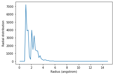
You may want to calculate the average RDF for a group of atoms where atoms overlap; for instance, looking at residue 60 around itself. In this case you should avoid including contributions from atoms interacting with themselves. The exclusion_block keyword allows you to mask pairs within the same chunk of atoms. Here you can pass exclusion_block=(1, 1) to create chunks of size 1 and avoid computing the RDF to itself.

irdf2 = rdf.InterRDF(res60, res60,
                     exclusion_block=(1, 1))
irdf2.run()

<MDAnalysis.analysis.rdf.InterRDF at 0x7fee87dbfed0>

plt.plot(irdf2.bins, irdf2.rdf)
plt.xlabel('Radius (angstrom)')
plt.ylabel('Radial distribution')

Text(0, 0.5, 'Radial distribution')

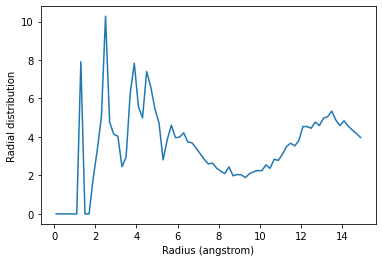
Similarly, you can apply this to residues.

thr = u.select_atoms('resname THR')
print('There are {} THR residues'.format(len(thr.residues)))
print('THR has {} atoms'.format(len(thr.residues[0].atoms)))

There are 11 THR residues
THR has 14 atoms

The code below calculates the RDF only using contributions from pairs of atoms where the two atoms are not in the same threonine residue.

irdf3 = rdf.InterRDF(thr, thr,
                     exclusion_block=(14, 14))
irdf3.run()

<MDAnalysis.analysis.rdf.InterRDF at 0x7fee87aa7e50>

plt.plot(irdf3.bins, irdf3.rdf)
plt.xlabel('Radius (angstrom)')
plt.ylabel('Radial distribution')

Text(0, 0.5, 'Radial distribution')

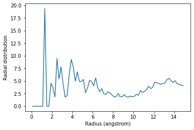
If you are splitting a residue over your two selections, you can discount pairs from the same residue by choosing appropriately sized exclusion blocks.

first = thr.residues[0]
print('THR has these atoms: ', ', '.join(first.atoms.names))
thr_c1 = first.atoms.select_atoms('name C*')
print('THR has {} carbons'.format(len(thr_c1)))
thr_other1 = first.atoms.select_atoms('not name C*')
print('THR has {} non carbons'.format(len(thr_other1)))

THR has these atoms:  N, H, CA, HA, CB, HB, OG1, HG1, CG2, HG21, HG22, HG23, C, O
THR has 4 carbons
THR has 10 non carbons

The exclusion_block here ensures that the RDF is only computed from threonine carbons to atoms in different threonine residues.

thr_c = thr.select_atoms('name C*')
thr_other = thr.select_atoms('not name C*')

irdf4 = rdf.InterRDF(thr_c, thr_other,
                     exclusion_block=(4, 10))
irdf4.run()

<MDAnalysis.analysis.rdf.InterRDF at 0x7fee8807db10>

plt.plot(irdf4.bins, irdf4.rdf)
plt.xlabel('Radius (angstrom)')
plt.ylabel('Radial distribution')

Text(0, 0.5, 'Radial distribution')

References

[1] Richard J. Gowers, Max Linke, Jonathan Barnoud, Tyler J. E. Reddy, Manuel N. Melo, Sean L. Seyler, Jan Domański, David L. Dotson, Sébastien Buchoux, Ian M. Kenney, and Oliver Beckstein. MDAnalysis: A Python Package for the Rapid Analysis of Molecular Dynamics Simulations. Proceedings of the 15th Python in Science Conference, pages 98–105, 2016. 00152. URL: https://conference.scipy.org/proceedings/scipy2016/oliver_beckstein.html, doi:10.25080/Majora-629e541a-00e.

[2] Naveen Michaud-Agrawal, Elizabeth J. Denning, Thomas B. Woolf, and Oliver Beckstein. MDAnalysis: A toolkit for the analysis of molecular dynamics simulations. Journal of Computational Chemistry, 32(10):2319–2327, July 2011. 00778. URL: http://doi.wiley.com/10.1002/jcc.21787, doi:10.1002/jcc.21787.