Principal component analysis of a trajectory
Here we compute the principal component analysis of a trajectory.
Last updated: February 2020
Minimum version of MDAnalysis: 0.17.0
Packages required:
Optional packages for visualisation:
[1]:
import MDAnalysis as mda
from MDAnalysis.tests.datafiles import PSF, DCD
from MDAnalysis.analysis import pca, align
import numpy as np
import pandas as pd
import matplotlib.pyplot as plt

import nglview as nv
import warnings
# suppress some MDAnalysis warnings about writing PDB files
warnings.filterwarnings('ignore')
%matplotlib inline
Loading files
The test files we will be working with here feature adenylate kinase (AdK), a phosophotransferase enzyme. ([BDPW09]) The trajectory DCD samples a transition from a closed to an open conformation.
[2]:
u = mda.Universe(PSF, DCD)
Principal component analysis
Principal component analysis (PCA) is a statistical technique that decomposes a system of observations into linearly uncorrelated variables called principal components. These components are ordered so that the first principal component accounts for the largest variance in the data, and each following component accounts for lower and lower variance. PCA is often applied to molecular dynamics trajectories to extract the large-scale conformational motions or “essential dynamics” of a protein. The frame-by-frame conformational fluctuation can be considered a linear combination of the essential dynamics yielded by the PCA.
In MDAnalysis, the method implemented in the PCA class (API docs) is as follows:
Optionally align each frame in your trajectory to the first frame.
Construct a 3N x 3N covariance for the N atoms in your trajectory. Optionally, you can provide a mean; otherwise the covariance is to the averaged structure over the trajectory.
Diagonalise the covariance matrix. The eigenvectors are the principal components, and their eigenvalues are the associated variance.
Sort the eigenvalues so that the principal components are ordered by variance.
Note
Principal component analysis algorithms are deterministic, but the solutions are not unique. For example, you could easily change the sign of an eigenvector without altering the PCA. Different algorithms are likely to produce different answers, due to variations in implementation. MDAnalysis may not return the same values as another package.
Warning
For best results, your trajectory should be aligned on your atom group selection before you run the analysis. Setting align=True will not give correct results in the PCA.
[3]:
aligner = align.AlignTraj(u, u, select='backbone',
                          in_memory=True).run()
You can choose how many principal components to save from the analysis with n_components. The default value is None, which saves all of them. You can also pass a mean reference structure to be used in calculating the covariance matrix. With the default value of None, the covariance uses the mean coordinates of the trajectory.
[4]:
pc = pca.PCA(u, select='backbone',
             align=False, mean=None,
             n_components=None).run()
The principal components are saved in pc.p_components. If you kept all the components, you should have an array of shape \((n_{atoms}\times3, n_{atoms}\times3)\).
[5]:
backbone = u.select_atoms('backbone')
n_bb = len(backbone)
print('There are {} backbone atoms in the analysis'.format(n_bb))
print(pc.p_components.shape)
There are 855 backbone atoms in the analysis
(2565, 2565)
The variance of each principal component is in pc.variance. For example, to get the variance explained by the first principal component:
[6]:
pc.variance[0]
[6]:
4203.190260100008
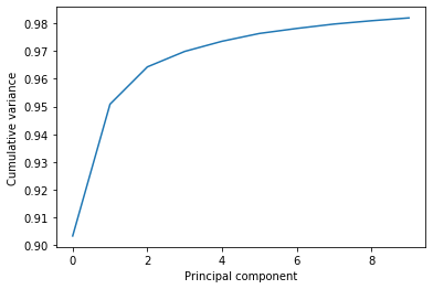
This variance is somewhat meaningless by itself. It is much more intuitive to consider the variance of a principal component as a percentage of the total variance in the data. MDAnalysis also tracks the percentage cumulative variance in pc.cumulated_variance. As shown below, the first principal component contains 90.3% the total trajectory variance. The first three components combined account for 96.4% of the total variance.
[7]:
print(pc.cumulated_variance[0])
print(pc.cumulated_variance[2])
0.9033944836257074
0.9642450284513093
[8]:
plt.plot(pc.cumulated_variance[:10])
plt.xlabel('Principal component')
plt.ylabel('Cumulative variance');
Visualising projections into a reduced dimensional space
The pc.transform() method transforms a given atom group into weights \(\mathbf{w}_i\) over each principal component \(i\).
\(\mathbf{r}(t)\) are the atom group coordinates at time \(t\), \(\mathbf{\overline{r}}\) are the mean coordinates used in the PCA, and \(\mathbf{u}_i\) is the \(i\)th principal component eigenvector \(\mathbf{u}\).
While the given atom group must have the same number of atoms that the principal components were calculated over, it does not have to be the same group.
Again, passing n_components=None will tranform your atom group over every component. Below, we limit the output to projections over 5 principal components only.
[9]:
transformed = pc.transform(backbone, n_components=5)
transformed.shape
[9]:
(98, 5)
The output has the shape (n_frames, n_components). For easier analysis and plotting we can turn the array into a DataFrame.
[10]:
df = pd.DataFrame(transformed,
                  columns=['PC{}'.format(i+1) for i in range(5)])
df['Time (ps)'] = df.index * u.trajectory.dt
df.head()
[10]:
| PC1 | PC2 | PC3 | PC4 | PC5 | Time (ps) | |
|---|---|---|---|---|---|---|
| 0 | 118.408403 | 29.088239 | 15.746624 | -8.344273 | -1.778052 | 0.0 |
| 1 | 115.561875 | 26.786799 | 14.652497 | -6.621619 | -0.629777 | 1.0 |
| 2 | 112.675611 | 25.038767 | 12.920275 | -4.324424 | -0.160540 | 2.0 |
| 3 | 110.341464 | 24.306985 | 11.427097 | -3.891525 | -0.173275 | 3.0 |
| 4 | 107.584299 | 23.464155 | 11.612103 | -2.293161 | -1.500821 | 4.0 |
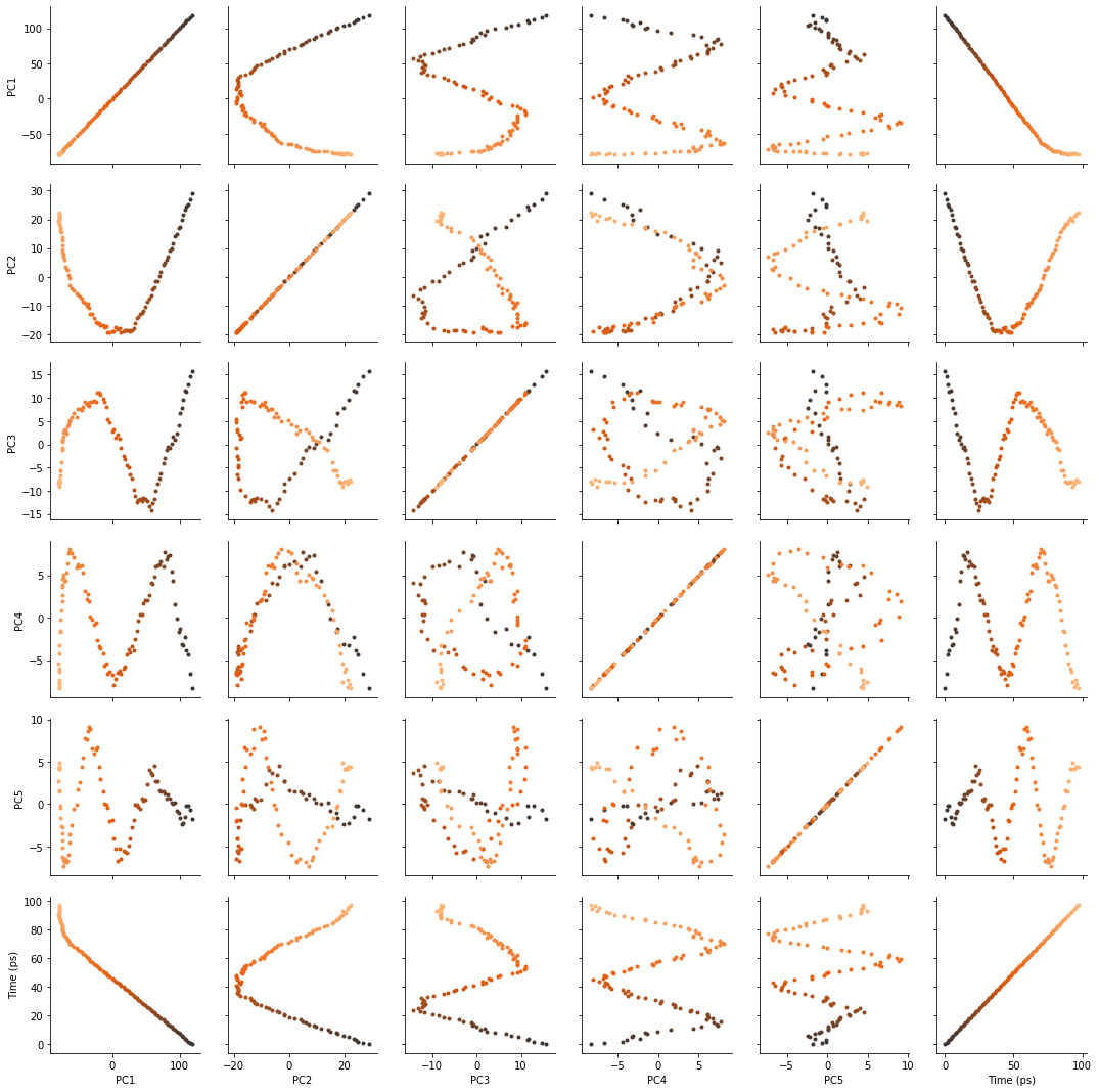
There are several ways we can visualise the data. Using the Seaborn’s PairGrid tool is the quickest and easiest way, if you have seaborn already installed.
Note
You will need to install the data visualisation library Seaborn for this function.
[11]:
import seaborn as sns

g = sns.PairGrid(df, hue='Time (ps)',
                 palette=sns.color_palette('Oranges_d',
                                           n_colors=len(df)))
g.map(plt.scatter, marker='.')
[11]:
<seaborn.axisgrid.PairGrid at 0x12b94bac8>
Another way to investigate the essential motions of the trajectory is to project the original trajectory onto each of the principal components, to visualise the motion of the principal component. The product of the weights \(\mathbf{w}_i(t)\) for principal component \(i\) with the eigenvector \(\mathbf{u}_i\) describes fluctuations around the mean on that axis, so the projected trajectory \(\mathbf{r}_i(t)\) is simply the fluctuations added onto the mean positions \(\mathbf{\overline{r}}\).
Below, we generate the projected coordinates of the first principal component. The mean positions are stored at pc.mean.
[12]:
pc1 = pc.p_components[:, 0]
trans1 = transformed[:, 0]
projected = np.outer(trans1, pc1) + pc.mean
coordinates = projected.reshape(len(trans1), -1, 3)
We can create a new universe from this to visualise the movement over the first principal component.
[13]:
proj1 = mda.Merge(backbone)
proj1.load_new(coordinates, order="fac")
[13]:
<Universe with 855 atoms>
[14]:
view = nv.show_mdanalysis(proj1.atoms)
view
If you have nglview installed, you can view the trajectory in the notebook. Otherwise, you can write the trajectory out to a file and use another program such as VMD. Below, we create a movie of the component.
[15]:
from nglview.contrib.movie import MovieMaker
movie = MovieMaker(view, output='pc1.gif', in_memory=True)
movie.make()

References
[1] Oliver Beckstein, Elizabeth J. Denning, Juan R. Perilla, and Thomas B. Woolf. Zipping and Unzipping of Adenylate Kinase: Atomistic Insights into the Ensemble of Open↔Closed Transitions. Journal of Molecular Biology, 394(1):160–176, November 2009. 00107. URL: https://linkinghub.elsevier.com/retrieve/pii/S0022283609011164, doi:10.1016/j.jmb.2009.09.009.
[2] Richard J. Gowers, Max Linke, Jonathan Barnoud, Tyler J. E. Reddy, Manuel N. Melo, Sean L. Seyler, Jan Domański, David L. Dotson, Sébastien Buchoux, Ian M. Kenney, and Oliver Beckstein. MDAnalysis: A Python Package for the Rapid Analysis of Molecular Dynamics Simulations. Proceedings of the 15th Python in Science Conference, pages 98–105, 2016. 00152. URL: https://conference.scipy.org/proceedings/scipy2016/oliver_beckstein.html, doi:10.25080/Majora-629e541a-00e.
[3] Naveen Michaud-Agrawal, Elizabeth J. Denning, Thomas B. Woolf, and Oliver Beckstein. MDAnalysis: A toolkit for the analysis of molecular dynamics simulations. Journal of Computational Chemistry, 32(10):2319–2327, July 2011. 00778. URL: http://doi.wiley.com/10.1002/jcc.21787, doi:10.1002/jcc.21787.