Analysing pore dimensions with HOLE

Here we use HOLE to analyse pore dimensions in a membrane.

Last executed: Feb 10, 2020 with MDAnalysis 1.0.0

Last updated: January 2020

Minimum version of MDAnalysis: 0.18.0

Packages required:

• MDAnalysis ([MADWB11], [GLB+16])

• MDAnalysisTests

• HOLE

• matplotlib

• numpy

Note

The classes in MDAnalysis.analysis.hole are wrappers around the HOLE program. Please cite ([SGW93], [SNW+96]) when using this module in published work.

import MDAnalysis as mda
from MDAnalysis.tests.datafiles import PDB_HOLE
from MDAnalysis.analysis import hole
import matplotlib.pyplot as plt
%matplotlib inline

Using HOLE with a PDB file

MDAnalysis.analysis.hole.HOLE is a wrapper class (API docs) that calls the HOLE program. This means you must have installed the program yourself before you can use the class. You then need to pass the path to your hole executable to the class; in this example, hole is installed at ~/hole2/exe/hole.

HOLE defines a series of points throughout the pore from which a sphere can be generated that does not overlap any atom (as defined by its van der Waals radius). (Please see ([SGW93], [SNW+96]) for a complete explanation). By default, it ignores residues with the following names: “SOL”, “WAT”, “TIP”, “HOH”, “K”, “NA”, “CL”. You can change these with the ignore_residues keyword. Note that the residue names must have 3 characters. Wildcards do not work.

The PDB file here is the experimental structure of the Gramicidin A channel. Note that we pass HOLE a PDB file directly, without creating a MDAnalysis.Universe.

h = hole.HOLE(PDB_HOLE, executable='~/hole2/exe/hole',
              logfile='hole1.out',
              sphpdb='hole1.sph',
              raseed=31415)
h.run()
h.collect()

This will create several outputs in your directory:

• hole1.out: the log file for HOLE.

• hole1.sph: a PDB-like file containing the coordinates of the pore centers.

• simple2.rad: file of Van der Waals’ radii

• run_n/radii_n_m.dat.gz: the profile for each frame

• tmp/pdb_name.pdb: the short name of a PDB file with your structure. As hole is a FORTRAN77 program, it is limited in how long of a filename that it can read.

The pore profile itself is in a dictionary at h.profiles. There is only one frame in this PDB file, so it is at h.profiles[0].

len(h.profiles[0])

425

Each profile is a numpy.recarray with the fields below as an entry for each rxncoord:

• frame: the integer frame number

• rxncoord: the distance along the pore axis in angstrom

• radius: the pore radius in angstrom

h.profiles[0].dtype.names

('frame', 'rxncoord', 'radius')

You can then proceed with your own analysis of the profiles.

rxncoords = h.profiles[0].rxncoord
pore_length = rxncoords[-1] - rxncoords[0]
print('The pore is {} angstroms long'.format(pore_length))

The pore is 42.4 angstroms long

Both HOLE and HOLEtraj (below) have the min_radius() function, which will return the minimum radius in angstrom for each frame. The resulting array has the shape (#n_frames, 2).

h.min_radius()

array([[0.     , 1.19707]])

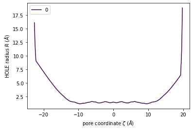
The class has a convenience plot() method to plot the coordinates of your pore.

h.plot();

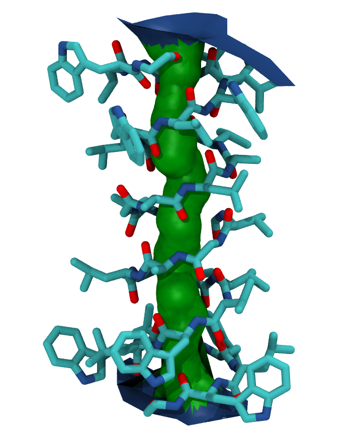
You can also create a VMD surface from the hole1.sph output file, using the create_vmd_surface function.

h.create_vmd_surface(filename='hole1.vmd')

'hole1.vmd'

To view this, open your PDB file in VMD.

vmd tmp*/*.pdb

Load the output file in Extensions > Tk Console:

source hole1.vmd

Your pore surface will be drawn as below.

MDAnalysis supports many of the options that can be customised in HOLE. For example, you can specify a starting point for the pore search within the pore with cpoint, and a sample distance (default: 0.2 angstrom) for the distance between the planes used in HOLE. Please see the MDAnalysis.analysis.hole for more information.

Using HOLE with a trajectory

One of the limitations of the hole program is that it can only accept PDB files. In order to use other formats with hole, or to run hole on trajectories, we can use the hole.HOLEtraj class with an MDAnalysis.Universe. While the example file below is a PDB, you can use any files to create your Universe.

from MDAnalysis.tests.datafiles import MULTIPDB_HOLE

u = mda.Universe(MULTIPDB_HOLE)

ht = hole.HOLEtraj(u, executable='~/hole2/exe/hole',
                   logfile='hole2.out',
                   sphpdb='hole2.sph')
ht.run()

Note that you do not need call collect() after calling run() with HOLEtraj. Again, the data is stored in ht.profiles as a dictionary of numpy.recarrays. The dictionary is indexed by frame; we can see the HOLE profile for the fourth frame below (truncated to 19.1126 angstrom from the pore axis). In this case, the frame field of each recarray is always 0.

ht.profiles[3][:10]

rec.array([(0, -23.6126, 15.98192), (0, -23.5126, 14.41088),
           (0, -23.4126, 12.88757), (0, -23.3126, 11.90096),
           (0, -23.2126, 11.27921), (0, -23.1126, 11.02236),
           (0, -23.0126, 10.96035), (0, -22.9126, 10.86575),
           (0, -22.8126, 10.77124), (0, -22.7126, 10.67909)],
          dtype=[('frame', '<i4'), ('rxncoord', '<f8'), ('radius', '<f8')])

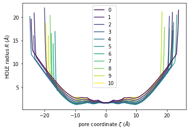
Again, plot() can plot the HOLE radius over each pore coordinate, differentiating each frame with colour.

ht.plot();

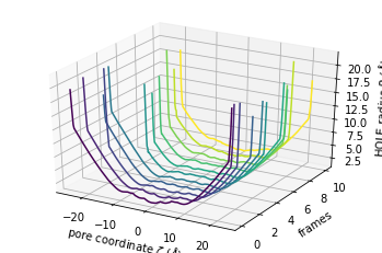
The plot3D() function separates each frame onto its own axis in a 3D plot.

ht.plot3D();

Ordering HOLE profiles with an order parameter

If you are interested in the HOLE profiles over an order parameter, you can directly pass that into the analysis. Below, we use an order parameter of RMSD from a reference structure.

Note

Please cite ([SFSB14]) when using the orderparameter functionality.

from MDAnalysis.analysis import rms

ref = mda.Universe(PDB_HOLE)
rmsd = rms.RMSD(u, ref, select='protein', weights='mass').run()
rmsd_values = rmsd.rmsd[:, 2]
rmsd_values

array([6.10501252e+00, 4.88398472e+00, 3.66303524e+00, 2.44202454e+00,
       1.22100521e+00, 1.67285541e-07, 1.22100162e+00, 2.44202456e+00,
       3.66303410e+00, 4.88398478e+00, 6.10502262e+00])

You can pass this in as orderparameter. The result profiles dictionary will have your order parameters as keys. You should be careful with this if your order parameter has repeated values, as duplicate keys are not possible; each duplicate key just overwrites the previous value.

ht2 = hole.HOLEtraj(u, executable='~/hole2/exe/hole',
                    logfile='hole3.out',
                    sphpdb='hole3.sph',
                    orderparameters=rmsd_values)
ht2.run()
ht2.profiles.keys()

odict_keys([6.105012519709198, 4.883984723991125, 3.663035235691455, 2.4420245432434005, 1.2210052104208637, 1.6728554140225013e-07, 1.2210016190719406, 2.4420245634673616, 3.6630340992950225, 4.883984778674993, 6.105022620520391])

You can see here that the dictionary does not order the entries by the order parameter. If you iterate over the class, it will return each (key, value) pair in sorted key order.

for order_parameter, profile in ht2:
    print(order_parameter, len(profile))

1.6728554140225013e-07 427
1.2210016190719406 389
1.2210052104208637 411
2.4420245432434005 421
2.4420245634673616 389
3.6630340992950225 383
3.663035235691455 423
4.883984723991125 419
4.883984778674993 369
6.105012519709198 455
6.105022620520391 401

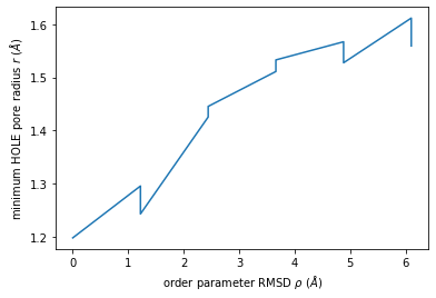
We can use this to plot the minimum radius as a function of RMSD from the reference structure.

import numpy as np
import matplotlib.pyplot as plt

min_radius = [[rmsd_i, p.radius.min()] for rmsd_i, p in ht2]
arr = np.array(min_radius)

plt.plot(arr[:, 0], arr[:, 1])
plt.xlabel(r"order parameter RMSD $\rho$ ($\AA$)")
plt.ylabel(r"minimum HOLE pore radius $r$ ($\AA$)");

References

[1] Richard J. Gowers, Max Linke, Jonathan Barnoud, Tyler J. E. Reddy, Manuel N. Melo, Sean L. Seyler, Jan Domański, David L. Dotson, Sébastien Buchoux, Ian M. Kenney, and Oliver Beckstein. MDAnalysis: A Python Package for the Rapid Analysis of Molecular Dynamics Simulations. Proceedings of the 15th Python in Science Conference, pages 98–105, 2016. 00152. URL: https://conference.scipy.org/proceedings/scipy2016/oliver_beckstein.html, doi:10.25080/Majora-629e541a-00e.

[2] Naveen Michaud-Agrawal, Elizabeth J. Denning, Thomas B. Woolf, and Oliver Beckstein. MDAnalysis: A toolkit for the analysis of molecular dynamics simulations. Journal of Computational Chemistry, 32(10):2319–2327, July 2011. 00778. URL: http://doi.wiley.com/10.1002/jcc.21787, doi:10.1002/jcc.21787.

[3] O S Smart, J M Goodfellow, and B A Wallace. The pore dimensions of gramicidin A. Biophysical Journal, 65(6):2455–2460, December 1993. 00522. URL: https://www.ncbi.nlm.nih.gov/pmc/articles/PMC1225986/, doi:10.1016/S0006-3495(93)81293-1.

[4] O. S. Smart, J. G. Neduvelil, X. Wang, B. A. Wallace, and M. S. Sansom. HOLE: a program for the analysis of the pore dimensions of ion channel structural models. Journal of Molecular Graphics, 14(6):354–360, 376, December 1996. 00935. doi:10.1016/s0263-7855(97)00009-x.

[5] Lukas S. Stelzl, Philip W. Fowler, Mark S. P. Sansom, and Oliver Beckstein. Flexible gates generate occluded intermediates in the transport cycle of LacY. Journal of Molecular Biology, 426(3):735–751, February 2014. 00000. URL: https://asu.pure.elsevier.com/en/publications/flexible-gates-generate-occluded-intermediates-in-the-transport-c, doi:10.1016/j.jmb.2013.10.024.