Evaluating convergence
Here we evaluate the convergence of a trajectory using the clustering ensemble similarity method and the dimensionality reduction ensemble similarity methods.
Last updated: December 2022 with MDAnalysis 2.4.0-dev0
Last updated: December 2022
Minimum version of MDAnalysis: 1.0.0
Packages required:
MDAnalysisTests
Optional packages for visualisation:
Note
The metrics and methods in the encore module are from ([TPB+15]). Please cite them when using the MDAnalysis.analysis.encore module in published work.
[1]:
import numpy as np
import matplotlib.pyplot as plt
%matplotlib inline

import MDAnalysis as mda
from MDAnalysis.tests.datafiles import PSF, DCD
from MDAnalysis.analysis import encore
from MDAnalysis.analysis.encore.clustering import ClusteringMethod as clm
from MDAnalysis.analysis.encore.dimensionality_reduction import DimensionalityReductionMethod as drm
Loading files
The test files we will be working with here feature adenylate kinase (AdK), a phosophotransferase enzyme. ([BDPW09])
[2]:
u = mda.Universe(PSF, DCD)
/home/pbarletta/mambaforge/envs/guide/lib/python3.9/site-packages/MDAnalysis/coordinates/DCD.py:165: DeprecationWarning: DCDReader currently makes independent timesteps by copying self.ts while other readers update self.ts inplace. This behavior will be changed in 3.0 to be the same as other readers. Read more at https://github.com/MDAnalysis/mdanalysis/issues/3889 to learn if this change in behavior might affect you.
  warnings.warn("DCDReader currently makes independent timesteps"
Evaluating convergence with similarity measures
The convergence of the trajectory is evaluated by the similarity of the conformation ensembles in windows of the trajectory. The trajectory is divided into windows that increase by window_size frames. For example, if your trajectory had 13 frames and you specified a window_size=3, your windows would be:
- Window 1: ---
- Window 2: ------
- Window 3: ---------
- Window 4: -------------
Where - represents 1 frame.
These are compared using either the similarity of their clusters (ces_convergence) or their reduced dimension coordinates (dres_convergence). The rate at which the similarity values drop to 0 is indicative of how much the trajectory keeps on resampling the same regions of the conformational space, and therefore is the rate of convergence.
Using default arguments with clustering ensemble similarity
See clustering_ensemble_similarity.ipynb for an introduction to comparing trajectories via clustering. See the API documentation for ces_convergence for more information.
[3]:
ces_conv = encore.ces_convergence(u,  # universe
                                  10,  # window size
                                  select='name CA')  # default
The output is an array of similarity values, with the shape (number_of_windows, number_of_clustering_methods).
[4]:
for row in ces_conv:
    for sim in row:
        print("{:>7.4f}".format(sim))
 0.4819
 0.4028
 0.3170
 0.2522
 0.1983
 0.1464
 0.0991
 0.0567
 0.0000
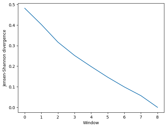
This can be easily plotted as a line.
[15]:
ces_fig, ces_ax = plt.subplots()
plt.plot(ces_conv)
ces_ax.set_xlabel('Window')
ces_ax.set_ylabel('Jensen-Shannon divergence')
[15]:
Text(0, 0.5, 'Jensen-Shannon divergence')
Comparing different clustering methods
You may want to try different clustering methods, or use different parameters within the methods. encore.ces_convergence allows you to pass a list of clustering_methods to be applied, much like normal clustering ensemble similarity methods.
Note
To use the other ENCORE methods available, you need to install scikit-learn.
The KMeans clustering algorithm separates samples into \(n\) groups of equal variance, with centroids that minimise the inertia. You must choose how many clusters to partition. (See the scikit-learn user guide for more information.)
[6]:
km1 = clm.KMeans(12,  # no. clusters
                 init = 'k-means++',  # default
                 algorithm="auto")    # default

km2 = clm.KMeans(6,  # no. clusters
                 init = 'k-means++',  # default
                 algorithm="auto")    # default

km3 = clm.KMeans(3,  # no. clusters
                 init = 'k-means++',  # default
                 algorithm="auto")    # default
When we pass a list of clustering methods to encore.ces_convergence, the similarity values get saved in ces_conv2 in order.
[7]:
ces_conv2 = encore.ces_convergence(u,  # universe
                                  10,  # window size
                                  select='name CA',
                                  clustering_method=[km1, km2, km3]
                                 )
ces_conv2.shape
[7]:
(9, 3)
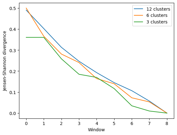
As you can see, the number of clusters partitioned by KMeans has an effect on the resulting rate of convergence.
[8]:
labels = ['12 clusters', '6 clusters', '3 clusters']

ces_fig2, ces_ax2 = plt.subplots()
for data, label in zip(ces_conv2.T, labels):
    plt.plot(data, label=label)
ces_ax2.set_xlabel('Window')
ces_ax2.set_ylabel('Jensen-Shannon divergence')
plt.legend()
[8]:
<matplotlib.legend.Legend at 0x7f9eb2146160>
Using default arguments with dimension reduction ensemble similarity
See dimension_reduction_ensemble_similarity.ipynb for an introduction on comparing trajectories via dimensionality reduction. We now use the dres_convergence function (API docs).
[9]:
dres_conv = encore.dres_convergence(u,  # universe
                                  10,  # window size
                                  select='name CA')  # default
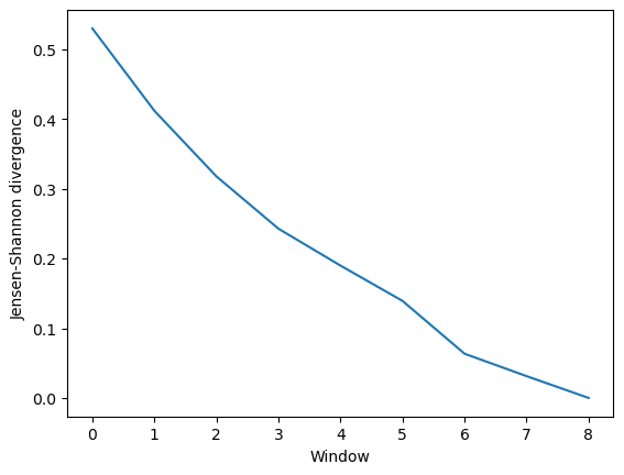
Much like ces_convergence, the output is an array of similarity values.
[10]:
dres_conv
[10]:
array([[0.52983036],
       [0.41177493],
       [0.31770319],
       [0.24269804],
       [0.18980852],
       [0.13913721],
       [0.06342056],
       [0.03125632],
       [0.        ]])
[11]:
dres_fig, dres_ax = plt.subplots()
plt.plot(dres_conv)
dres_ax.set_xlabel('Window')
dres_ax.set_ylabel('Jensen-Shannon divergence')
[11]:
Text(0, 0.5, 'Jensen-Shannon divergence')
Comparing different dimensionality reduction methods
Again, you may want to compare the performance of different methods.
Principal component analysis uses singular value decomposition to project data onto a lower dimensional space. (See the scikit-learn user guide for more information.)
The method provided by MDAnalysis.encore accepts any of the keyword arguments of sklearn.decomposition.PCA except n_components. Instead, use dimension to specify how many components to keep.
[12]:
pc1 = drm.PrincipalComponentAnalysis(dimension=1,
                                     svd_solver='auto')
pc2 = drm.PrincipalComponentAnalysis(dimension=2,
                                     svd_solver='auto')
pc3 = drm.PrincipalComponentAnalysis(dimension=3,
                                     svd_solver='auto')
[13]:
dres_conv2 = encore.dres_convergence(u,  # universe
                                  10,  # window size
                                  select='name CA',
                                  dimensionality_reduction_method=[pc1, pc2, pc3]
                                 )
dres_conv2.shape
[13]:
(9, 3)
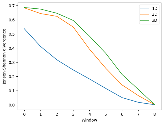
Again, the size of the subspace you choose to include in your similarity comparison, affects the apparent rate of convergence over the trajectory.
[14]:
labels = ['1D', '2D', '3D']

dres_fig2, dres_ax2 = plt.subplots()
for data, label in zip(dres_conv2.T, labels):
    plt.plot(data, label=label)
dres_ax2.set_xlabel('Window')
dres_ax2.set_ylabel('Jensen-Shannon divergence')
plt.legend()
[14]:
<matplotlib.legend.Legend at 0x7f9e98499ee0>
References
[1] Oliver Beckstein, Elizabeth J. Denning, Juan R. Perilla, and Thomas B. Woolf. Zipping and Unzipping of Adenylate Kinase: Atomistic Insights into the Ensemble of Open↔Closed Transitions. Journal of Molecular Biology, 394(1):160–176, November 2009.
URL: https://linkinghub.elsevier.com/retrieve/pii/S0022283609011164, doi:10.1016/j.jmb.2009.09.009.
[2] Richard J. Gowers, Max Linke, Jonathan Barnoud, Tyler J. E. Reddy, Manuel N. Melo, Sean L. Seyler, Jan Domański, David L. Dotson, Sébastien Buchoux, Ian M. Kenney, and Oliver Beckstein. MDAnalysis: A Python Package for the Rapid Analysis of Molecular Dynamics Simulations. Proceedings of the 15th Python in Science Conference, pages 98–105, 2016.
URL: https://conference.scipy.org/proceedings/scipy2016/oliver_beckstein.html, doi:10.25080/Majora-629e541a-00e.
[3] Naveen Michaud-Agrawal, Elizabeth J. Denning, Thomas B. Woolf, and Oliver Beckstein. MDAnalysis: A toolkit for the analysis of molecular dynamics simulations. Journal of Computational Chemistry, 32(10):2319–2327, July 2011.
URL: http://doi.wiley.com/10.1002/jcc.21787, doi:10.1002/jcc.21787.
[4] Matteo Tiberti, Elena Papaleo, Tone Bengtsen, Wouter Boomsma, and Kresten Lindorff-Larsen. ENCORE: Software for Quantitative Ensemble Comparison. PLOS Computational Biology, 11(10):e1004415, October 2015.
URL: https://journals.plos.org/ploscompbiol/article?id=10.1371/journal.pcbi.1004415, doi:10.1371/journal.pcbi.1004415.