Comparing the geometric similarity of trajectories
Here we compare the geometric similarity of trajectories using the following path metrics:
the Hausdorff distance
the discrete Fréchet
Last updated: December 2022 with MDAnalysis 2.4.0-dev0
Last updated: December 2022
Minimum version of MDAnalysis: 0.18.0
Packages required:
Optional packages for visualisation:
Note
The metrics and methods in the psa path similarity analysis module are from ([SKTB15]). Please cite them when using the MDAnalysis.analysis.psa module in published work.
[1]:
import numpy as np
import matplotlib.pyplot as plt
%matplotlib inline

import MDAnalysis as mda
from MDAnalysis.tests.datafiles import (PSF, DCD, DCD2, GRO, XTC,
                                        PSF_NAMD_GBIS, DCD_NAMD_GBIS,
                                        PDB_small, CRD)
from MDAnalysis.analysis import psa
import warnings
# suppress some MDAnalysis warnings about writing PDB files
warnings.filterwarnings('ignore')
Loading files
The test files we will be working with here feature adenylate kinase (AdK), a phosophotransferase enzyme. ([BDPW09])
[2]:
u1 = mda.Universe(PSF, DCD)
u2 = mda.Universe(PSF, DCD2)
u3 = mda.Universe(GRO, XTC)
u4 = mda.Universe(PSF_NAMD_GBIS, DCD_NAMD_GBIS)
u5 = mda.Universe(PDB_small, CRD, PDB_small,
                  CRD, PDB_small, CRD, PDB_small)

ref = mda.Universe(PDB_small)


labels = ['DCD', 'DCD2', 'XTC', 'NAMD', 'mixed']
The trajectories can have different lengths, as seen below.
[3]:
print(len(u1.trajectory), len(u2.trajectory), len(u3.trajectory))
98 102 10
Aligning trajectories
We set up the PSAnalysis (API docs) with our list of Universes and labels. While path_select determines which atoms to calculate the path similarities for, select determines which atoms to use to align each Universe to reference.
[4]:
CORE_sel = 'name CA and (resid 1:29 or resid 60:121 or resid 160:214)'

ps = psa.PSAnalysis([u1, u2, u3, u4, u5],
                    labels=labels,
                    reference=ref,
                    select=CORE_sel,
                    path_select='name CA')
Generating paths
For each Universe, we will generate a transition path containing each conformation from a trajectory using generate_paths (API docs).
First, we will do a mass-weighted alignment of each trajectory to the reference structure reference, along the atoms in select. To turn off the mass weighting, set weights=None. If your trajectories are already aligned, you can skip the alignment with align=False.
[5]:
ps.generate_paths(align=True, save=False, weights='mass')
Hausdorff method
Now we can compute the similarity of each path. The default metric is to use the Hausdorff method. [5] The Hausdorff distance between two conformation transition paths \(P\) and \(Q\) is:
\(\delta_h(P|Q)\) is the directed Hausdorff distance from \(P\) to \(Q\), and is defined as:
The directed Hausdorff distance of \(P\) to \(Q\) is the distance between the two points, \(p \in P\) and its structural nearest neighbour \(q \in Q\), for the point \(p\) where the distance is greatest. This is not commutative, i.e. the directed Hausdorff distance from \(Q\) to \(P\) is not the same. (See scipy.spatial.distance.directed_hausdorff for more information).
In MDAnalysis, the Hausdorff distance is the RMSD between a pair of conformations in \(P\) and \(Q\), where the one of the conformations in the pair has the least similar nearest neighbour.
[6]:
ps.run(metric='hausdorff')
The distance matrix is saved in ps.D.
[7]:
ps.D
[7]:
array([[ 0.        ,  1.33312648, 22.37206002,  2.04737477,  7.55204678],
       [ 1.33312648,  0.        , 22.3991666 ,  2.07957562,  7.55032598],
       [22.37206002, 22.3991666 ,  0.        , 22.42282661, 25.74534554],
       [ 2.04737477,  2.07957562, 22.42282661,  0.        ,  7.67052252],
       [ 7.55204678,  7.55032598, 25.74534554,  7.67052252,  0.        ]])
Plotting
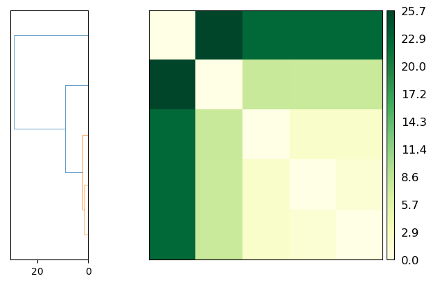
psa.PSAnalysis provides two convenience methods for plotting this data. The first is to plot a heat-map dendrogram from clustering the trajectories based on their path similarity. You can use any clustering method supported by scipy.cluster.hierarchy.linkage; the default is ‘ward’.
[8]:
fig = ps.plot(linkage='ward')
<Figure size 640x480 with 0 Axes>
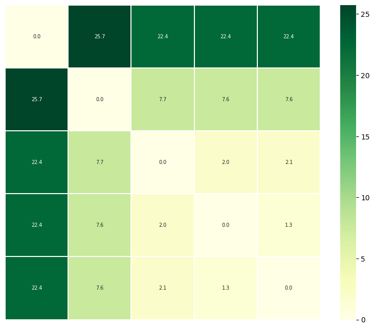
The other is to plot a heatmap annotated with the distance values. Again, the trajectories are displayed in an arrangement that fits the clustering method.
Note
You will need to install the data visualisation library Seaborn for this function.
[9]:
fig = ps.plot_annotated_heatmap(linkage='single')
<Figure size 640x480 with 0 Axes>
Discrete Fréchet distances
The discrete Fréchet distance between two conformation transition paths \(P\) and \(Q\) is:
where \(C\) is a coupling in the set of all couplings \(\Gamma_{P,Q}\) between \(P\) and \(Q\). A coupling \(C(P,Q)\) is a sequence of pairs of conformations in \(P\) and \(Q\), where the first/last pairs are the first/last points of the respective paths, and for each successive pair, at least one point in \(P\) or \(Q\) must advance to the next frame.
The coupling distance \(\|C\|\) is the largest distance between a pair of points in such a sequence.
In MDAnalysis, the discrete Fréchet distance is the lowest possible RMSD between a conformation from \(P\) and a conformation from \(Q\), where the two frames are at similar points along the trajectory, and they are the least structurally similar in that particular coupling sequence. [6-9]
[10]:
ps.run(metric='discrete_frechet')
ps.D
[10]:
array([[ 0.        ,  1.33312649, 22.37205967,  2.04737475,  7.55204694],
       [ 1.33312649,  0.        , 22.39916723,  2.07957565,  7.55032613],
       [22.37205967, 22.39916723,  0.        , 22.42282569, 25.74534511],
       [ 2.04737475,  2.07957565, 22.42282569,  0.        ,  7.67052241],
       [ 7.55204694,  7.55032613, 25.74534511,  7.67052241,  0.        ]])
Plotting
[11]:
fig = ps.plot(linkage='ward')
<Figure size 640x480 with 0 Axes>

[12]:
fig = ps.plot_annotated_heatmap(linkage='single')
<Figure size 640x480 with 0 Axes>

References
[1] Oliver Beckstein, Elizabeth J. Denning, Juan R. Perilla, and Thomas B. Woolf. Zipping and Unzipping of Adenylate Kinase: Atomistic Insights into the Ensemble of Open↔Closed Transitions. Journal of Molecular Biology, 394(1):160–176, November 2009.
URL: https://linkinghub.elsevier.com/retrieve/pii/S0022283609011164, doi:10.1016/j.jmb.2009.09.009.
[2] Richard J. Gowers, Max Linke, Jonathan Barnoud, Tyler J. E. Reddy, Manuel N. Melo, Sean L. Seyler, Jan Domański, David L. Dotson, Sébastien Buchoux, Ian M. Kenney, and Oliver Beckstein. MDAnalysis: A Python Package for the Rapid Analysis of Molecular Dynamics Simulations. Proceedings of the 15th Python in Science Conference, pages 98–105, 2016.
URL: https://conference.scipy.org/proceedings/scipy2016/oliver_beckstein.html, doi:10.25080/Majora-629e541a-00e.
[3] Naveen Michaud-Agrawal, Elizabeth J. Denning, Thomas B. Woolf, and Oliver Beckstein. MDAnalysis: A toolkit for the analysis of molecular dynamics simulations. Journal of Computational Chemistry, 32(10):2319–2327, July 2011.
URL: http://doi.wiley.com/10.1002/jcc.21787, doi:10.1002/jcc.21787.
[4] Sean L. Seyler, Avishek Kumar, M. F. Thorpe, and Oliver Beckstein. Path Similarity Analysis: A Method for Quantifying Macromolecular Pathways. PLOS Computational Biology, 11(10):e1004568, October 2015. URL: https://dx.plos.org/10.1371/journal.pcbi.1004568, doi:10.1371/journal.pcbi.1004568.